R de jeu #2 : Happy new yeaR

Eh oui, 2017 est déjà (presque) fini… À l’heure qu’il est, on boucle les derniers dossiers de l’année, et on se prépare psychologiquement à aller célébrer la nouvelle année comme il se doit. Bref, “pas le temps de niaiser” comme le disent si bien nos amis d’outre-Atlantique.

Histoire de se changer les idées avant de décoller, nous vous avons concocté un deuxième volet de R de jeu, avec la thématique fin d’année !

All I want for Christmas is data

Se connecter à Spotify, on l’a déjà fait, on ne va pas vous en reparler 😉

[pastacode lang=”R” manual=”library(httr)%0Aapp_id%20%3C-%20%22app_spotify%22%0Aclient_id%20%3C-%20%22***%22%0Aclient_secret%20%3C-%20%22***%22%0Aspoti_ep%20%3C-%20httr%3A%3Aoauth_endpoint(%0A%20%20authorize%20%3D%20%22https%3A%2F%2Faccounts.spotify.com%2Fauthorize%22%2C%0A%20%20access%20%3D%20%22https%3A%2F%2Faccounts.spotify.com%2Fapi%2Ftoken%22)%0Aspoti_app%20%3C-%20httr%3A%3Aoauth_app(app_id%2C%20client_id%2C%20client_secret)%0Aaccess_token%20%3C-%20httr%3A%3Aoauth2.0_token(spoti_ep%2C%20spoti_app%2C%20scope%20%3D%20%22user-read-private%22)” message=”” highlight=”” provider=”manual”/]

Hop, une bonne chose de faite. On va se faire une petite recherche avec la thématique New Year, vous en pensez quoi ?

[pastacode lang=”R” manual=”tracks%20%3C-%20GET(%22https%3A%2F%2Fapi.spotify.com%2Fv1%2Fsearch%3Fq%3Dnew%2520year%26type%3Dtrack%22%2C%20%0A%20%20%20%20config(token%20%3D%20access_token)%2C%20query%20%3D%20list(limit%20%3D%2050))%0Acontent(tracks)%24tracks%24total%0A%5B1%5D%2035890″ message=”” highlight=”” provider=”manual”/]

Est-ce que Spotify va nous laisser aller chercher tout ça ? On a le droit d’y aller 50 par 50… lançons le test 🙂

[pastacode lang=”R” manual=”library(tidyverse)%0Alibrary(jsonlite)%0Aget_tracks%20%3C-%20function(offset)%7B%0A%20%20print(offset)%0A%20%20api_res%20%3C-%20GET(%22https%3A%2F%2Fapi.spotify.com%2Fv1%2Fsearch%3Fq%3Dnew%2520year%26type%3Dtrack%22%2C%20%0A%20%20%20%20%20%20%20%20config(token%20%3D%20access_token)%2C%20query%20%3D%20list(limit%20%3D%2050%2C%20offset%20%3D%20offset))%0A%20%20played%20%3C-%20api_res%24content%20%25%3E%25%20rawToChar()%20%25%3E%25%20fromJSON(flatten%20%3D%20TRUE)%20%0A%20%20return(as_tibble(played%24tracks%24items))%0A%7D%20%0Asafe_tracks%20%3C-%20safely(get_tracks)%0Anew_year_songs%20%3C-%20map(seq(0%2C%2035890%2C%2050)%2C%20safe_tracks)%0Aclean_songs%20%3C-%20new_year_songs%20%25%3E%25%20map(%22result%22)%20%25%3E%25%20compact()%20%25%3E%25%20bind_rows()%0Adim(clean_songs)%0A%5B1%5D%2035890%20%20%20%2025″ message=”” highlight=”” provider=”manual”/]

Il semblerait qu’on ait réussi à toutes les avoir !

[pastacode lang=”R” manual=”clean_songs%20%3C-%20select(clean_songs%2C%20artists%2C%20duration_ms%2C%20explicit%2C%20%0A%20%20%20%20name%2C%20popularity%2C%20type%2C%20album.name)” message=”” highlight=”” provider=”manual”/]

Visualisation

Il nous faudrait une petite palette de couleurs spécialement prévue pour le Nouvel An, non ? Aller, on va emprunter celles de Color-Hex.

[pastacode lang=”R” manual=”library(rvest)%0Alibrary(glue)%0A%0Aget_palettes_list%20%3C-%20function(search)%7B%0A%20%20search%20%3C-%20URLencode(search)%0A%20%20read_html(glue(%22http%3A%2F%2Fwww.color-hex.com%2Fcolor-palettes%2F%3Fkeyword%3D%7Bsearch%7D%22))%20%25%3E%25%0A%20%20%20%20html_nodes(%22.palettecontainerlist%20a%22)%20%25%3E%25%0A%20%20%20%20html_attr(%22href%22)%20%25%3E%25%0A%20%20%20%20stringr%3A%3Astr_extract_all(%22(%5B0-9%5D%2B)%22)%20%25%3E%25%0A%20%20%20%20as_vector()%0A%7D%0A%0Alist_palettes%20%3C-%20get_palettes_list(%22new%20year%22)%0A%0Aget_palette%20%3C-%20function(page)%7B%0A%20%20Sys.sleep(0.5)%0A%20%20read_html(glue(%22http%3A%2F%2Fwww.color-hex.com%2Fcolor-palette%2F%7Bpage%7D%22))%20%25%3E%25%0A%20%20html_table()%20%25%3E%25%0A%20%20modify_depth(1%2C%20%22Hex%22)%20%25%3E%25%0A%20%20as_vector()%0A%7D%0Afull_palette%20%3C-%20map(list_palettes%2C%20get_palette)%20%25%3E%25%20as_vector()%20%25%3E%25%20%0A%20%20%20%20unique()%20%25%3E%25%20discard(%C2%A0~%20.x%20%3D%3D%20%22ffffff%22)%0Afull_palette%0A%20%5B1%5D%20%22%23000934%22%20%22%231624a1%22%20%22%23a2bdf2%22%20%22%23fc5b8d%22%20%22%23a8026e%22%0A%20%5B6%5D%20%22%23f90000%22%20%22%239a1010%22%20%22%23f4eb1a%22%20%22%23e1d921%22%20%22%23e79516%22%0A%5B11%5D%20%22%23000000%22%20%22%23cfcfcf%22%20%22%2314054c%22%20%22%23fffff0%22%20%22%23ffd376%22%0A%5B16%5D%20%22%23ffe700%22%20%22%23c900ff%22%20%22%232f00ff%22%20%22%23ff00c1%22%20%22%237cff00%22″ message=”” highlight=”” provider=”manual”/]

On a de quoi faire…

Maintenant, allons regarder rapidement ce qu’il se trame dans ce dataset ? Des tracks plutôt populaires ?

[pastacode lang=”R” manual=”library(ggthemes)%0Aggplot(clean_songs)%20%2B%0A%20%20aes(x%20%3D%20popularity)%20%2B%0A%20%20geom_density(fill%20%3D%20sample(palette%2C%201))%20%2B%20%0A%20%20labs(title%20%3D%20%22Popularit%C3%A9%20des%20tracks%20du%20nouvel%20an%22%2C%20%0A%20%20%20%20%20%20%20subtitle%20%3D%20%22donn%C3%A9es%20via%20Spotify%22%2C%20%0A%20%20%20%20%20%20%20x%20%3D%20%22Popularit%C3%A9%22%2C%20%0A%20%20%20%20%20%20%20y%20%3D%20%22Densit%C3%A9%22%2C%20%0A%20%20%20%20%20%20%20caption%20%3D%20%22thinkr.fr%22)%20%2B%20%0A%20%20theme_few()” message=”” highlight=”” provider=”manual”/]

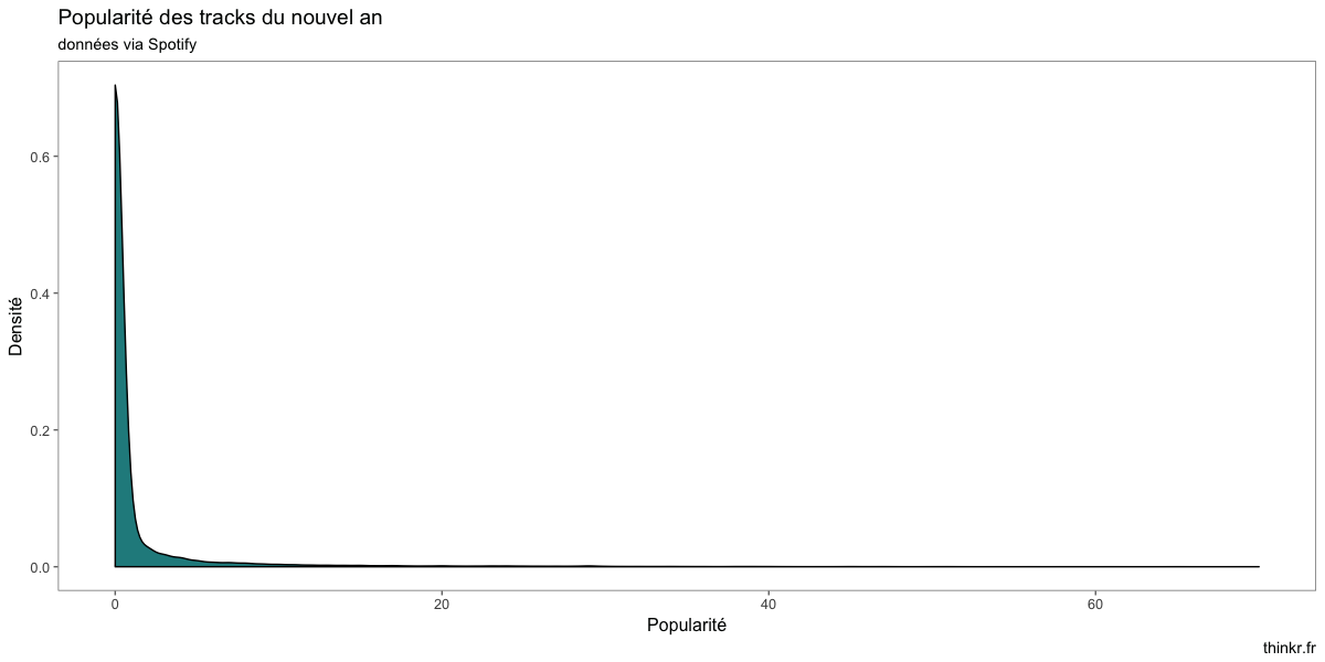
À première vue, quelques morceaux populaires, et un paquet de morceaux moins populaires. Lesquels sont en top de liste ?

[pastacode lang=”R” manual=”clean_songs%20%25%3E%25%0A%20%20select(name%2C%20popularity)%20%25%3E%25%0A%20%20top_n(10)%20%25%3E%25%0A%20%20knitr%3A%3Akable()” message=”” highlight=”” provider=”manual”/]

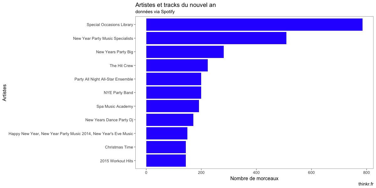
Et les artistes les plus présents dans notre jeu de données ?

[pastacode lang=”R” manual=”clean_songs%20%25%3E%25%20%0A%20%20count(artists%2C%20sort%20%3D%20TRUE)%20%25%3E%25%20%0A%20%20top_n(10)%20%25%3E%25%0A%20%20ggplot()%20%2B%0A%20%20aes(reorder(artists%2C%20n)%2C%20n)%20%2B%0A%20%20geom_col(fill%20%3D%20sample(full_palette%2C%201))%20%2B%20%0A%20%20coord_flip()%20%2B%20%0A%20%20labs(title%20%3D%20%22Artistes%20et%20tracks%20du%20nouvel%20an%22%2C%20%0A%20%20%20%20%20%20%20subtitle%20%3D%20%22donn%C3%A9es%20via%20Spotify%22%2C%20%0A%20%20%20%20%20%20%20x%20%3D%20%22Artistes%22%2C%20%0A%20%20%20%20%20%20%20y%20%3D%20%22Nombre%20de%20morceaux%22%2C%20%0A%20%20%20%20%20%20%20caption%20%3D%20%22thinkr.fr%22)%20%2B%20%0A%20%20theme_few()” message=”” highlight=”” provider=”manual”/]

Maintenant, on se ferait bien une fonction de recommandation de playlist, non ? Disons, une fonction qui permet de créer une playlist adaptée au temps qu’on veut y passer. Commençons par une fonction qui va sampler jusqu’à atteindre un certain niveau :

[pastacode lang=”R” manual=”sample_until%3C-%20function(tbl%2C%20col%2C%20threshold)%7B%0A%20%20%0A%20%20col%20%3C-%20enquo(col)%0A%20%20vec%20%3C-%20pull(tbl%2C%20!!%20col)%20%0A%20%20%0A%20%20if%20(%20min(vec)%20%3E%20threshold%20)%20stop(%22Impossible%20de%20trouver%20une%20combinaison%20pour%20ce%20threshold%22)%0A%20%20%0A%20%20res%20%3C-%20sample_n(tbl%2C%201)%0A%20%20while(%20sum(%20pull(res%2C%20!!%20col)%20)%20%3C%20threshold)%20%7B%0A%20%20%20%20%20res%20%3C-%20bind_rows(res%2C%20sample_n(tbl%2C%201))%20%25%3E%25%20distinct()%0A%20%20%20%7D%0A%20%20res%0A%7D%0A%0Asample_until(iris%2C%20Sepal.Length%2C%2030)%20%25%3E%25%20knitr%3A%3Akable()” message=”” highlight=”” provider=”manual”/]

Et voilà ! Combinons maintenant ça avec notre jeu de données de chansons :

[pastacode lang=”R” manual=”clean_songs%24artists%20%3C-%20modify_depth(clean_songs%24artists%2C%201%2C%20~%20.x%24name)%20%25%3E%25%20%0A%20%20%20%20modify_depth(1%2C%20~%20paste(.x%2C%20collapse%20%3D%20’%2C%20′))%20%25%3E%25%20%0A%20%20%20%20as_vector()%0A%0Amake_me_a_playlist%20%3C-%20function(duree_s%2C%20popularite_max%2C%20explicit_filter%20%3D%20FALSE)%7B%0A%20%20duree_milli%20%3C-%20duree_s%20*%201000%0A%20%20good%20%3C-%20clean_songs%20%25%3E%25%0A%20%20%20%20filter(popularity%20%3C%3D%20popularite_max)%20%0A%20%20if(explicit_filter)%20good%20%3C-%20filter(good%2C%20!%20explicit)%20%0A%20%20sample_until(good%2C%20duration_ms%2C%20duree_milli)%20%25%3E%25%20%0A%20%20%20%20select(artists%2C%20name%2C%20duration_ms)%20%25%3E%25%20knitr%3A%3Akable()%0A%7D%0Amake_me_a_playlist(600%2C%2050)” message=”” highlight=”” provider=”manual”/]

\o/

À la recherche de la soirée parfaite

C’est bien beau d’avoir une belle playlist, mais il serait mieux de trouver un endroit pour jouer ces morceaux. Qu’est-ce que nous propose Facebook ?

[pastacode lang=”R” manual=”get_event%20%3C-%20function(fb_url)%7B%0A%20%20res%20%3C-%20GET(fb_url)%0A%20%20res%20%3C-%20content(res)%0A%20%20return(list(id%20%3D%20map(res%24data%2C%20%22id%22)%2C%20paging%20%3D%20res%24paging))%0A%7D%0A%0A%23%20La%20premi%C3%A8re%20page%20%3A%0A%23%20Le%20token%20est%20temporaire%2C%20%C3%A7a%20ne%20marchera%20pas%20chez%20vous%20%3B)%0Ares%20%3C-%20get_event(%22https%3A%2F%2Fgraph.facebook.com%2Fv2.11%2Fsearch%3Fq%3Dnew%2520year%26type%3Devent%26access_token%3DEAACEdEose0cBAEwhntvjdDENCoU19y3He5q7L6cHoyL9J3RkpxuZCHGxXxN2UZCfFO5d7Ng90MnMh8lbnSP8cZA71iked9ZBLr6wrredSmGCZCY7BgwIXUGEEd0PRdyuD8lhymPdEJjB413T6fqGra0rQ4Wzb3l23auncQDE2xl5cVpgqyIiBAcazYzbFVo8ZD%22)%0A%0Anext_page%20%3C-%20try(res%24paging%24%60next%60)%0Aid_list%20%3C-%20res%24id%0A%0Awhile(%20length(next_page)%20!%3D%200%20)%20%7B%0A%20%20res%20%3C-%20get_event(next_page)%0A%20%20next_page%20%3C-%20try(res%24paging%24%60next%60)%0A%20%20id_list%20%3C-%20c(id_list%2C%20res%24id)%0A%7D” message=”” highlight=”” provider=”manual”/]

76 événements, c’est plutôt pas mal. On va scraper tout ça !

[pastacode lang=”R” manual=”event_details%20%3C-%20function(id)%7B%0A%20%20fromJSON(glue(%22https%3A%2F%2Fgraph.facebook.com%2Fv2.11%2F%7Bid%7D%3Faccess_token%3DEAACEdEose0cBAEwhntvjdDENCoU19y3He5q7L6cHoyL9J3RkpxuZCHGxXxN2UZCfFO5d7Ng90MnMh8lbnSP8cZA71iked9ZBLr6wrredSmGCZCY7BgwIXUGEEd0PRdyuD8lhymPdEJjB413T6fqGra0rQ4Wzb3l23auncQDE2xl5cVpgqyIiBAcazYzbFVo8ZD%22))%0A%7D%0Aall_events%20%3C-%20map(id_list%2C%20event_details)” message=”” highlight=”” provider=”manual”/]

Comme souvent lorsque l’on appelle des API, nous avons une liste irrégulière (en JSON, non-tabulaire), que nous avons besoin de transformer en tableau. Go pour une fonction qui réglera ça !

[pastacode lang=”R” manual=”library(lubridate)%0Atibble_that%20%3C-%20function(list)%7B%0A%20%20tibble(desc%20%3D%20list%24description%20%25%7C%7C%25%20NA%2C%20%0A%20%20%20%20%20%20%20%20%20start_time%20%3D%20ymd_hms(list%24start_time)%20%25%7C%7C%25%20NA%2C%0A%20%20%20%20%20%20%20%20%20end_time%20%3D%20ymd_hms(list%24end_time)%20%25%7C%7C%25%20NA%2C%0A%20%20%20%20%20%20%20%20%20name%20%3D%20list%24name%20%25%7C%7C%25%20NA%2C%0A%20%20%20%20%20%20%20%20%20place%20%3D%20list%24place%24name%20%25%7C%7C%25%20NA%2C%0A%20%20%20%20%20%20%20%20%20city%20%3D%20list%24place%24location%24city%20%25%7C%7C%25%20NA%2C%0A%20%20%20%20%20%20%20%20%20country%20%3D%20list%24place%24location%24country%20%25%7C%7C%25%20NA%2C%0A%20%20%20%20%20%20%20%20%20street%20%3D%20list%24place%24location%24street%20%25%7C%7C%25%20NA%2C%0A%20%20%20%20%20%20%20%20%20zip%20%3D%20list%24place%24location%24zip%20%25%7C%7C%25%20NA%2C%0A%20%20%20%20%20%20%20%20%20placeid%20%3D%20list%24place%24id%20%25%7C%7C%25%20NA%0A%20%20)%0A%7D%0Aevents%20%3C-%20map_df(all_events%2C%20tibble_that)” message=”” highlight=”” provider=”manual”/]

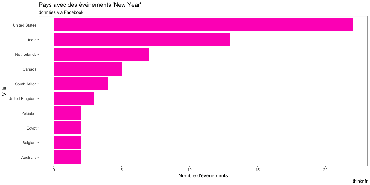
Alors, quels pays peut-on viser ?

[pastacode lang=”R” manual=”library(lubridate)%0Atibble_that%20%3C-%20function(list)%7B%0A%20%20tibble(desc%20%3D%20list%24description%20%25%7C%7C%25%20NA%2C%20%0A%20%20%20%20%20%20%20%20%20start_time%20%3D%20ymd_hms(list%24start_time)%20%25%7C%7C%25%20NA%2C%0A%20%20%20%20%20%20%20%20%20end_time%20%3D%20ymd_hms(list%24end_time)%20%25%7C%7C%25%20NA%2C%0A%20%20%20%20%20%20%20%20%20name%20%3D%20list%24name%20%25%7C%7C%25%20NA%2C%0A%20%20%20%20%20%20%20%20%20place%20%3D%20list%24place%24name%20%25%7C%7C%25%20NA%2C%0A%20%20%20%20%20%20%20%20%20city%20%3D%20list%24place%24location%24city%20%25%7C%7C%25%20NA%2C%0A%20%20%20%20%20%20%20%20%20country%20%3D%20list%24place%24location%24country%20%25%7C%7C%25%20NA%2C%0A%20%20%20%20%20%20%20%20%20street%20%3D%20list%24place%24location%24street%20%25%7C%7C%25%20NA%2C%0A%20%20%20%20%20%20%20%20%20zip%20%3D%20list%24place%24location%24zip%20%25%7C%7C%25%20NA%2C%0A%20%20%20%20%20%20%20%20%20placeid%20%3D%20list%24place%24id%20%25%7C%7C%25%20NA%0A%20%20)%0A%7D%0Aevents%20%3C-%20map_df(all_events%2C%20tibble_that)” message=”” highlight=”” provider=”manual”/]

[pastacode lang=”R” manual=”events%20%25%3E%25%0A%20%20count(city)%20%25%3E%25%0A%20%20na.omit()%20%25%3E%25%0A%20%20top_n(5)%20%25%3E%25%0A%20%20arrange(desc(n))%20%25%3E%25%0A%20%20ggplot()%20%2B%20%0A%20%20aes(reorder(city%2C%20n)%2C%20n)%20%2B%20%0A%20%20geom_col(fill%20%3D%20sample(full_palette%2C%201))%20%2B%20%0A%20%20coord_flip()%20%2B%20%0A%20%20labs(title%20%3D%20%22Villes%20avec%20des%20%C3%A9v%C3%A9nements%20’New%20Year’%22%2C%20%0A%20%20%20%20%20%20%20subtitle%20%3D%20%22donn%C3%A9es%20via%20Facebook%22%2C%20%0A%20%20%20%20%20%20%20x%20%3D%20%22Ville%22%2C%20%0A%20%20%20%20%20%20%20y%20%3D%20%22Nombre%20d’%C3%A9v%C3%A9nements%22%2C%20%0A%20%20%20%20%20%20%20caption%20%3D%20%22thinkr.fr%22)%20%2B%20%0A%20%20theme_few()” message=”” highlight=”” provider=”manual”/]

Il va falloir qu’on voit ce qu’on a de plus proche. Petit tour du côté de l’API distance24 ?

[pastacode lang=”R” manual=”get_route%20%3C-%20function(from%2C%20to)%7B%0A%20%20if%20(is.na(to))%20%7B%0A%20%20%20%20return(NULL)%0A%20%20%7D%0A%20%20from_clean%20%3C-%20URLencode(from)%0A%20%20to_clean%20%3C-%20URLencode(to)%0A%20%20a%20%3C-%20GET(glue(%22http%3A%2F%2Ffr.distance24.org%2Froute.json%3Fstops%3D%7Bfrom_clean%7D%7C%7Bto_clean%7D%22))%0A%20%20tibble(from%20%3D%20from%2C%20%0A%20%20%20%20%20%20%20%20%20to%20%3D%20to%2C%20%0A%20%20%20%20%20%20%20%20%20dist%20%3D%20content(a)%24distances%5B%5B1%5D%5D)%0A%7D%0Atravel%20%3C-%20map_df(events%24city%2C%20~%20get_route(%22Rennes%22%2C%20.x))” message=”” highlight=”” provider=”manual”/]

Rendez-vous au plus proche :

[pastacode lang=”R” manual=”travel%20%25%3E%25%0A%20%20top_n(-%205)%20%25%3E%25%0A%20%20arrange(dist)%20%25%3E%25%0A%20%20knitr%3A%3Akable()” message=”” highlight=”” provider=”manual”/]

Direction Londres alors 😉

Les douze développeurs de minuit

Enfin, on a prévu de bouger… mais il se passe peut-être trop de choses sur GitHub ? Alerte #FOMO

[pastacode lang=”R” manual=”github_app%20%3C-%20oauth_app(%22github%22%2C%20%22***%22%2C%20%22***%22)%0A%0Aaccess_token%20%3C-%20oauth2.0_token(oauth_endpoints(%22github%22)%2C%20github_app)%0A%0Ares%20%3C-%20GET(url%20%3D%20%22https%3A%2F%2Fapi.github.com%2Fsearch%2Frepositories%3Fq%3Dnew%2Byear%26sort%3Dstars%26order%3Ddesc%22%2C%20config(token%20%3D%20access_token))%0A%0Acontent(res)%24total_count%0A%5B1%5D%201527″ message=”” highlight=”” provider=”manual”/]

[pastacode lang=”R” manual=”get_search%20%3C-%20function(page%2C%20search)%7B%0A%20%20Sys.sleep(2)%0A%20%20search%20%3C-%20URLencode(search)%0A%20%20res%20%3C-%20GET(url%20%3D%20glue(%22https%3A%2F%2Fapi.github.com%2Fsearch%2Frepositories%3Fq%3D%7Bsearch%7D%26per_page%3D100%26page%3D%7Bpage%7D%22)%2C%20%0A%20%20%20%20%20%20%20%20%20%20%20%20%20%20config(token%20%3D%20access_token))%0A%20%20%23%20Surveillons%20le%20rate%20limit%0A%20%20message(res%24headers%24%60x-ratelimit-remaining%60)%0A%20%20res%24content%20%25%3E%25%20rawToChar()%20%25%3E%25%20fromJSON()%20%25%3E%25%20.%24items%20%25%3E%25%20discard(is.data.frame)%0A%7D%0A%0Aall_github_ny%20%3C-%20map_df(.x%20%3D%201%3A15%2C%20.f%20%3D%20~%20get_search(.x%2C%20%22New%20Year%22))%0Adim(all_github_ny)%0A%5B1%5D%201000%20%20%2070″ message=”” highlight=”” provider=”manual”/]

Ah, c’est étrange, 1500 résultats et des bananes, et nous n’avons que les 1000 premiers résultats… On ne peut pas avoir la page 15 ?

[pastacode lang=”R” manual=”GET(url%20%3D%20glue(%22https%3A%2F%2Fapi.github.com%2Fsearch%2Frepositories%3Fq%3DNew%2520year%26per_page%3D100%26page%3D15%22)%2C%20%0A%20%20%20%20%20%20%20%20%20%20%20%20%20%20config(token%20%3D%20access_token))%0A%0AResponse%20%5Bhttps%3A%2F%2Fapi.github.com%2Fsearch%2Frepositories%3Fq%3DNew%2520year%26per_page%3D100%26page%3D15%5D%0A%20%20Date%3A%202017-12-27%2016%3A35%0A%20%20Status%3A%20422%0A%20%20Content-Type%3A%20application%2Fjson%3B%20charset%3Dutf-8%0A%20%20Size%3A%20134%20B%0A%7B%0A%20%20%22message%22%3A%20%22Only%20the%20first%201000%20search%20results%20are%20available%22%2C%0A%20%20%22documentation_url%22%3A%20%22https%3A%2F%2Fdeveloper.github.com%2Fv3%2Fsearch%2F%22%0A%7D” message=”” highlight=”” provider=”manual”/]

Ceci explique cela ! Seulement les 1000 premiers résultats sont renvoyés par l’API de Github !

Regardons un peu ce qu’il se trame dans ce jeu de données.

[pastacode lang=”R” manual=”all_github_ny%20%25%3E%25%0A%20%20count(language)%20%25%3E%25%0A%20%20na.omit()%20%25%3E%25%0A%20%20top_n(10)%20%25%3E%25%0A%20%20arrange(desc(n))%20%25%3E%25%0A%20%20ggplot()%20%2B%0A%20%20aes(reorder(language%2C%20n)%2C%20n)%20%2B%0A%20%20geom_col(fill%20%3D%20sample(full_palette%2C%201))%20%2B%20%0A%20%20coord_flip()%20%2B%20%0A%20%20labs(title%20%3D%20%22Langages%20sur%20Github%20pour%20’New%20Year’%22%2C%20%0A%20%20%20%20%20%20%20subtitle%20%3D%20%22donn%C3%A9es%20via%20GitHub%22%2C%20%0A%20%20%20%20%20%20%20x%20%3D%20%22Langages%22%2C%20%0A%20%20%20%20%20%20%20y%20%3D%20%22Nombre%20de%20repos%22%2C%20%0A%20%20%20%20%20%20%20caption%20%3D%20%22thinkr.fr%22)%20%2B%20%0A%20%20theme_few()” message=”” highlight=”” provider=”manual”/]

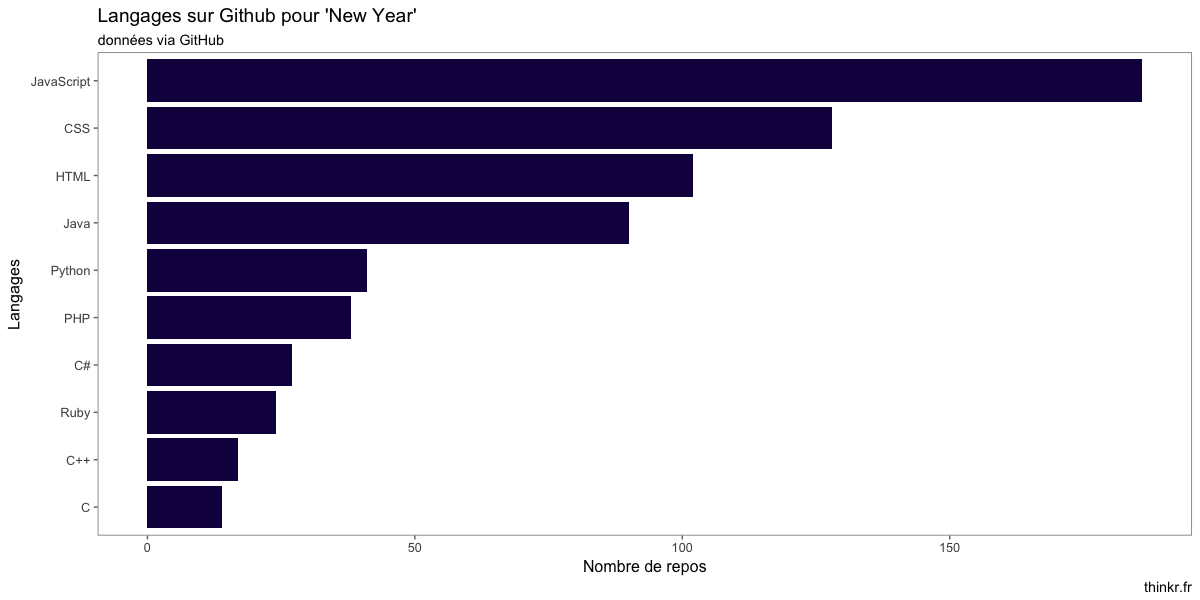Pas beaucoup de R, donc… et plutôt des langages orientés web…

[pastacode lang=”R” manual=”all_github_ny%20%25%3E%25%0A%20%20filter(language%20%3D%3D%20%22R%22)%20%25%3E%25%0A%20%20nrow()%0A%5B1%5D%205″ message=”” highlight=”” provider=”manual”/]

Alors, de quoi ça parle tout ça ?

[pastacode lang=”R” manual=”library(tidytext)%0Aall_github_ny%20%25%3E%25%0A%20%20unnest_tokens(word%2C%20description)%20%25%3E%25%0A%20%20anti_join(stop_words)%20%25%3E%25%0A%20%20count(word)%20%25%3E%25%20%0A%20%20na.omit()%20%25%3E%25%0A%20%20top_n(10)%20%25%3E%25%0A%20%20knitr%3A%3Akable()” message=”” highlight=”” provider=”manual”/]

Au final, pas mal d’application web en JavaScript, HTML et CSS pour le final countdown…

Allez, c’est pas tout, mais on a un Nouvel An à développer nous 😉